Introduction

I applied to 13 colleges across the United States, with a focus on engineering and technology schools. I spent the largest amount of time writing essays, and I submitted approximately 10,500 words overall. Instead of writing unique essays for every prompt, I tried to reuse as much as possible to make the process more efficient, and now that I’ve finished I want to know which of my essays were the most “reusable,” to gain a better idea of what colleges are generally interested in hearing from their applicants. This information is also relevant to students who are preparing to apply as it may help them decide how to build their résumé or plan their own essays.

To actually identify reusable essays, I wanted to build and visualize groups of similar essays using a graph. The window below shows nodes representing prompts and edges that indicate that the prompts’ responses share seven or more five-word phrases (5-grams). Thus, groups of connected nodes correspond to similar responses, and the largest groups correspond to the essays that were, in my case, the most reusable.

You can interact with the graph below:

Or, see the images here.

This post will explain the process of building this graph from my raw essays. I also wanted to calculate an adjusted word count that would reflect the number of unique words I submitted to see how many words I could actually reuse.

If you are a student, I have separated my advice/experience about the application process into another post, where I will take this information and explain how it’s actually relevant.

Planning Process

Part of the reason this problem is interesting to solve is because it boils down to a simple but robust problem: identify all shared sub-strings between members of a group of larger strings. This is also the central problem in plagiarism detection, which is where I started looking for methods to approach the problem. Plagiarised documents are frequently identified using a method called Fingerprinting in which specific sub-strings are selected as representatives, or “fingerprints,” of a document. If any two documents share a fingerprint, at least some parts of them are plagiarised.

Selecting fingerprints is like picking out the “important parts” of a document, and it makes plagiarism detection more efficient by directly reducing the amount of string comparisons required to detect shared sub-strings. Plus, the documents can be indexed by their fingerprints to make the process even more efficient: to evaluate a new document, you would only have to select its fingerprints and look them up in the index instead of checking it against every other document in the database.

Because of the relatively small amount of text to be considered in this case, I chose to make the process simpler by forgoing the fingerprint selection process and considering all of an essay’s fingerprint candidates as its representative, so I don’t have to do anything funky to guarantee that I find every possible substring match. Still, the idea of increasing the efficiency of the process by indexing documents by their substrings was central to this investigation, so I want to reiterate it:

Which of these diagrams makes it more obvious where two documents share fingerprints?

Implementation

This is the real meat of the project. I’m going to run through each step and explain what’s going on.

Preprocessing

Preprocessing is where the input text data (or corpus) gets cleaned before use. Not all of my preprocessing steps are shown here — the processes of exporting my essays to text and consolidating them in a JSON file through regex-fu is omitted on the grounds of boring and esoteric.

Anyways, we start with an array of JSON essay objects with the following members:

• college: which college is requesting the essay?
• prompt: the writing prompt
• maxwords: maximum word count for this essay (-1 if no maximum is provided)
• content: the actual content of the essay
• id: lastly, each essay gets a numeric identifier to help keep track of it

import json
from nltk.tokenize import word_tokenize
import re

essays_in = open("essays.json")
essays = json.loads(essays_in.read()) # Parse the json file into an object
essays_in.close() # Don't forget to close the file


has_chars = re.compile("[A-z]") # Match capital and lowercase letters 
for essay in essays:
    # Word_tokenize is imported above, and splits our document into words
    # To filter out punctuation, we apply filter() to tokens and remove those
    #   which don't match our regex
    pre_tokens = word_tokenize(essay["content"])
    pre_tokens = list(filter(has_chars.search, pre_tokens))
    # Afterwords, we update the essay object
    essay["tokens"] = pre_tokens
    essay["wordcount"] = len(pre_tokens)

# This will help us retrieve essays by their ids
id_to_idx = {e["id"]:idx for idx, e in enumerate(essays)}

In this step, the data is loaded and converted to tokens with the Natural Language Toolkit’s word_tokenize method. NLTK’s tokenizer uses some advanced methods (outside this post’s scope, but more info here) to split text into sentences first, and then into words. It is worth using in my opinion over (for example) splitting on spaces to avoid the edge cases that result from every day English text. It would be nice to have unambiguous sentence ending characters, but this language is too complex to work nicely.

Now, we can display some interesting information about the corpus:

from collections import defaultdict
words_submitted = defaultdict(int)

for essay in essays:
    words_submitted[essay["college"]] += essay["wordcount"]


words_submitted = sorted(words_submitted.items(), key = lambda x: x[1], reverse = True)

print("\n".join(["{0}. {1}: {2} words".format(idx + 1, *items) for idx, items in enumerate(words_submitted)]))

print( "\nTotal: {0} Words".format(sum([essay["wordcount"] for essay in essays])))
print("Essays Submitted: {0}".format(len(essays)))

1. Princeton: 1660 words
2. Berkeley: 1399 words
3. Stanford: 1224 words
4. Brown: 1060 words
5. MIT: 967 words
6. Harvard: 860 words
7. University of Washington: 802 words
8. Carnegie Mellon: 646 words
9. UW Honors College: 591 words
10. Rensselaer: 403 words
11. UCF Burnett Honors College: 383 words
12. Georgia Tech: 302 words
13. University of Central Florida: 259 words
14. Northeastern: 0 words
15. University of Florida: 0 words

Total: 10556 Words
Essays Submitted: 56

The word count is a bit off because the tokenizer doesn’t exactly split strings into perfect words, but it gives us a good place to start.

Analysis

After preprocessing, we can start analyzing the data. In this case, we’re going to need to do some work to get the information we’re interested in.

N-Grams

Before we start, there is an important concept to introduce. The plan was to come up with some “fingerprints” for each document, but we need to decide what those fingerprints will actually be.

Conceptually, we want matching fingerprints to indicate shared phrases, so they should correspond to groups of words in the original document. We’ll use a text processing staple: the n-gram. An n-gram is an ordered group of n items from some sample text. Depending on context, items can be words, individual characters, or other stuff… Here, we’ll use words to make it easy to compute the adjusted word count.

For example, the phrase “lorem ipsum dolor sit amet” has three 3-grams: (lorem ipsum dolor), (ipsum dolor sit), and (dolor sit amet).

Let’s make a method to automate the process of generating n-grams. I picked this up from Scott Triglia’s Blog, so credit goes to him for the great technique.

def ngrams(n, tokens):
    return zip(*[tokens[i:] for i in range(n)])

# Note that zip() returns a generator, which we must convert to a list to print nicely
print(list(ngrams(3, ["lorem", "ipsum", "dolor", "sit", "amet"])))

[('lorem', 'ipsum', 'dolor'), ('ipsum', 'dolor', 'sit'), ('dolor', 'sit', 'amet')]

This method is pretty, but it’s also very compact and difficult to understand at first. I think the most confusing part is the use of Python’s zip() method, which is pretty uncommon. Zip() takes an unlimited number of list inputs and returns a list generator whose first element is a tuple of all the first elements of the inputs, whose second element has all the second elements, and so on. The output list ends when the elements of the smallest input list have been exhausted. So, the list comprehension in our n-gram generator creates a series of successive token arrays each offset by one from the last, and then zips them. This process is actually very visually intuitive:

The decision to use n-grams for fingerprints still leaves one more choice for us to make. How do we set n, the length of our phrases?

The biggest effect n has is that it sets a threshold below which shared phrases will not be identified. If we represent documents using phrases that are n words long, we won’t match any phrases that are less than n characters. To see why, consider 3-grams that share a phrase with length below the threshold.

So, we want to choose n to eliminate extraneous matches between documents for things like idioms or buzzwords, but otherwise it should be as low as possible otherwise so that we catch all of the “important” phrases. I chose to set n arbitrarily at 5, but we’ll talk about some experimentation with different n values later.

Now, we’re going to simultaneously compute each essay’s 5-grams and build the index of which 5-grams occur in each essay. If you need a refresher, take another look at the two data structures from earlier. We’re going to assemble both the 5-grams for each essay (the left example) and the essays for each 5-gram (the right example).

n = 5

gram_to_hash = {} # This is a fake hash and I'm a hash fake-fan

# The default dict acts like a dictionary, but returns a default value
# for keys that haven't been assigned. Here, it is an empty list.
essays_by_hash = defaultdict(list)

for essay in essays:
    grams = list(ngrams(n, essay["tokens"])) # Generate our ngrams
    # ? But doesn't converting to list remove benefits of a generator?
    #     Yes, but we need to use the elements twice and otherwise we would
    #     exhaust the generator on the first use and be unable to use it again
    
    essay["ngrams"] = grams # Assign them to the essay - our left example
    
    for idx, gram in enumerate(grams):
        if not gram in gram_to_hash: # If the gram doesn't have a hash number assigned
            hno = len(gram_to_hash) # Hashes are assigned sequentially
            gram_to_hash[gram] = hno
            # Because our ngram function generates tuples, which are immutable,
            # we can use them as dictionary keys. Lists cannot do this.
        else:
            # If an ngram already has a hash number, we have to find it
            hno = gram_to_hash[gram]
            
        # Add the essay to the list of essays for each ngram hash - our right example
        # Because we used a defaultdict(list), we don't have to check that 
        #     the essay list already exists.
        # We are also tracking the position at which an ngram occurs with idx
        essays_by_hash[hno].append((essay["id"], idx))

# Once every ngram has a hash value, we will make a reverse index for convenience
hash_to_gram = {value: key for key, value in gram_to_hash.items() }

This is not actually as complicated as it looks. First off, I want to point out line 31:

essays_by_hash[hno].append((essay["id"], idx))

Here, for every 5-gram in an essay, we log that essay’s id and the position where that hash occurs. This will be important later, but it’s easy to forget about later.

The main idea for this block is generating “hash values” for each of our 5-grams and then tracking which essays have those has. A hash is a function that takes an input of arbitrary size and maps it to an output of fixed size (the hash value), with possible information loss. Think of using a cookie cutter to make shapes out of dough: you know the exact shape of the dough you take away, at the cost of leaving some of the dough behind.

Hashes are usually designed to minimize the probability that two inputs will share the same hash value, which is called a hash collision. If each hash number corresponds to one and only one input, it can serve as a unique identifier for that. Unfortunately, if there are more inputs than outputs, a collision is inevitable by the pigeonhole principle. Then one input would share the same hash number, and it is no longer unique.

To see how that idea applies to our situation, take a look at line 18 above:

if not gram in gram_to_hash

Checking for the existence of a 5-gram in our growing list every time we want to add a new one is really inefficient ( :^) ). If we had a hypothetical hash function to map arbitrary n-grams to integers, we could just skip this step by indexing each n-gram by its hash value. As long as we trust the unlikeliness of hash collisions, n-grams would only ever be overwritten by the same n-gram occurring later in the corpus.

For this project, I chose not to implement a hash function because I can afford to be inefficient when working with such small amounts of text. However, I’m still calling the 5-gram ID numbers hashes because I want to avoid any confusion between numbers associated with essays (IDs) and numbers associated with 5-grams (hashes).

So far, we’ve come up with “hash values” for each 5-gram, built a dictionary linking each hash to the essays it occurs in and, for each essay, the index where the first token in the 5-gram. For the sake of spotting edge cases, I also want to point out that if the same 5-gram were to occur twice in an essay, it would be added twice to the index with different position values. Now we can start using our 5-grams.

The Adjusted Word Count

During preprocessing, we calculated the word count token count, just for fun. Word counts are used frequently as direct indicators of document length, but they can also serve as proxy measurements for time spent on/work applied to the writing process. In my case, that relationship doesn’t hold because I reused essays and inflated the word count. So, let’s try to find an adjusted word count that more accurately reflects the number of unique words I wrote for my applications.

To make that idea more concrete, we want phrases that are used in multiple essays to contribute the same total number of words to an overall word count as if they were only used once. Then, mathematically, a five-word phrase occurring in $N$ essays should contribute $5 \cdot \frac{1}{N}$ words to the word count.

Phew, well, I know where we can find some five-word phrases — our 5-grams. We already know which essays they occur in, so the adjusted word count will be easy!

There is still one problem we have to consider: every n-gram in the dataset overlaps with others to guarantee examination of all possible five-word phrases. So, we have to consider which 5-grams should “take ownership” of words that belong to multiple to avoid counting too many words. We can avoid accidentally overlooking the occurrence of parts of a phrase in a document by giving the priority the phrases that occur the most, like so:

To see why this works, think about what might happen if we gave priority to the last 3-gram, (dolor, sit, amet). Since “amet” only occurs once, the phrase as a whole also only occurs once, so the appearances of “dolor” and “sit” in two other documents would be ignored. If any less frequent n-gram takes precedence over a more frequent n-gram, some word occurrences would have to be ignored, so priority must be given to the most frequent n-grams.

relationships = sorted(essays_by_hash.items(),
           reverse=True, key=lambda x: len(x[1])) # reverse=True makes the sort descending

The easiest way to give precedence to more frequent n-grams is to just consider them first. Then, if a specific 5-gram overlaps another 5-gram that we have already considered, we know it must be in more essays and that it should take ownership. In this statement, we take the (key, value) pairs that are returned from items() and sort them by the length of the second element. We are taking our index of hash numbers to essays containing those hashes and then converting it to a list generator, sorted so that the number of essays associated with each hash descends as you progress down the list.

Now, we can actually calculate how many words each 5-gram contributes to the essays it occurs in:

considered = []
substrs = []
for hno, essays_in in relationships: # Begin the progression down our list
    essay_contrib = [] # In this array, we will keep track of the words contributed by the 5-gram to each essay it occurs in
    for essay_group in essays_in:
        # Remember from when we built the essays_by_hash index that the hash numbers are stored with
        # the essay they occur in and the position where they occur. This lets us look in that 5-gram's
        # vicinity in each essay to check which words it "owns"
        essay_id = essay_group[0] 
        pos = essay_group[1]
        
        idx = id_to_idx[essay_id]
        e = essays[idx]
        
        words_contributed = n # Each phrase starts off with the words it owns
        # The most overlap two n-grams could have is if one occurs right after another
        # The least overlap would be if one occurs (n-1) tokens after another 
        for i in range(1, n): 
            if(len(e["ngrams"]) > (pos + i) and gram_to_hash[e["ngrams"][pos + i]] in considered):
                # If an n-gram that has already been considered overlaps with this one, the overlapped words don't count here
                words_contributed -= (n - i)
                break
        for i in range(1, n):
            if(0 <= (pos - i) and gram_to_hash[e["ngrams"][pos - i]] in considered):
                words_contributed -= (n - i)
                break
        # We have to correct negative word counts resulting from n-grams which are double overlapped
        if(words_contributed < 0): words_contributed = 0 
        essay_contrib.append(words_contributed) # Log the words contributed by this 5-gram to this essay
    # When a 5-gram has been considered in all of its essays, we will log that too
    considered.append(hno)
    substrs.append({"essays_in": essays_in, "words": essay_contrib, "hash_no": hno})

This is also not as complicated as it might seem. There is one inner loop and one outer loop to consider: for each 5-gram (the outer loop), for every essay containing that 5-gram (the inner loop), check for any overlap on that 5-gram in that essay and find how many words to add. The check for overlapping words is also simpler than it seems: using the position information we got a few steps ago, move outwards one index at a time (first checking all right indexes, then left indexes) in each essay. The earliest overlapping 5-grams on each side (if they exist) have precedence because they’ve already been considered, so we don’t count the words which are overlapped by subtracting their length:

Assuming everything worked correctly, the last step in piecing together the adjusted word counts is to add up the $\frac{1}{N}$ scaled substring word counts for each essay. However, that’s not an easy assumption, so we’ll prove it by also keeping track of the unscaled word counts for each essay. Then, we can compare them to our known word counts from the preprocessing step to verify that every essay’s words are accounted for.

test_wcs = defaultdict(int)
adj_wcs = defaultdict(int)

for shared_substr in substrs:
    # Remember that the words list for each substring is organized so that its elements correspond to the
    #     elements of the essays_in list of essays and positions. We toss out the position information with _
    #     and grab the rest
    for words_contrib_idx, (essay_id, _) in enumerate(shared_substr["essays_in"]):
        essay_idx = id_to_idx[essay_id]
        
        words_contrib = shared_substr["words"][words_contrib_idx] # Words contributed to the current essay 
        test_wcs[essay_idx] += words_contrib # Unscaled word count
        adj_wcs[essay_id] += (1 / len(shared_substr["words"])) * words_contrib # scaled word count

does_it_work = all([test_wcs[idx] == essays[idx]["wordcount"] for idx in id_to_idx.values() if essays[idx]["wordcount"] >= n])
print("Does it work: " + str(does_it_work))

Does it work: True

Jokes aside, tests are actually very important, and if this project weren’t for fun it would need a lot more of them.

This test isn’t even a great one — it has a (sort-of) caveat built in:

if essays[idx]["wordcount"] >= n

When I first wrote it, I spent way too long trying to figure out why it was failing. Evidently, I had forgotten why I used n-grams in the first place: to avoid matching phrases shorter than n words. That means the two adjectives Princeton wanted that describe me were too short to get any 5-grams, creating a word count inconsistency.

Anyways, since we appear to have calculated the other essays’ word counts correctly, we can check out how many unique words each college wanted. This block simply assigns each essay its adjusted wordcount and gets the total adjusted word count for each college.

college_adj_wordcount = defaultdict(int)

for essay_id, adj_wc in adj_wcs.items():
    # Assigning an adjusted word count to each essay
    idx = id_to_idx[essay_id]
    essays[idx]["adj_wordcount"] = adj_wc
    
for essay_id, adj_wc in adj_wcs.items():
    # Getting the total adjusted word count for each essay
    idx = id_to_idx[essay_id]
    college = essays[idx]["college"]
    college_adj_wordcount[college] += adj_wc

final_wcs = [(college, round(wc, 1)) for college, wc in college_adj_wordcount.items()]
final_wcs = sorted(final_wcs, key = lambda x: x[1], reverse = True)

print("\n".join(["{0}. {1}: {2} words".format(idx + 1, *items) for idx, items in enumerate(final_wcs)]))

print( "\nTotal: {0} Words".format(round(sum(college_adj_wordcount.values()), 2)))

1. Berkeley: 1114.3 words
2. Princeton: 1048.3 words
3. Stanford: 864.4 words
4. Brown: 692.1 words
5. University of Washington: 667.0 words
6. MIT: 597.7 words
7. UW Honors College: 586.2 words
8. Harvard: 400.6 words
9. Carnegie Mellon: 340.7 words
10. Georgia Tech: 302.0 words
11. Rensselaer: 224.1 words
12. UCF Burnett Honors College: 111.7 words
13. University of Central Florida: 82.5 words

Total: 7031.8 Words

The total adjusted word count is about 7,000 words. 10,500ish minus 7,000ish is 3,500ish reused words! It is also worth noting that the four largest applications in standard word count are still the four largest applications, in the same order, as under the adjusted word count. The longest applications have applicants answer more unique questions, so the order of the top of the list doesn’t really change.

Also, two members of the list from the beginning of this post aren’t here. They didn’t have a writing supplement, so they weren’t included in the shared substrings computations.

When I first started this project, I definitely didn’t expect the word count to be the most complicated part.

Finding the Most Valuable Prompt

Compared to the adjusted word count, this will be a piece of cake. Essays that have the same content share lots of phrases, so we can classify entire groups of essays as reused as long as they share a lot of phrases. We could do something like printing the largest essay groups, but a graph would make a much better visualization.

from graphviz import Graph

# This method will automatically insert line breaks every n words to make the graph look nicer
def line_breaks(text, n):
    # n for number of words per line
    words = text.split(" ") # wow lame-o doesn't even use nltk.tokenize.word_tokenize
    return "\n".join([" ".join(words[i * n:(i+1) * n]) for i in range((len(words) // n) + 1)])

# Note the balance here between setting N to be very high and just filtering here
dot = Graph(comment = "College Essays", format="svg", engine="dot")
edges = defaultdict(int)
for essay in essays:
    if(essay["prompt"]): # Filter out 0 length essays
        # Nodes are identified by the essay's ID
        # And labeled by the college and the essay prompt
        dot.node(str(essay["id"]), line_breaks("{0}: {1}".format(essay["college"], essay["prompt"]), 7))
    for gram in essay["ngrams"]: 
        # For every essay, check what other essays share its ngrams and keep track of the relationship
        for essay_id, _ in essays_by_hash[gram_to_hash[gram]]:
            if essay_id > essay["id"]: # this is to avoid mutual relationships (a-b and b-a) as well as essay to itself relationships
                edges[(str(essay_id), str(essay["id"]))] += 1
                
# An edge is formed if two essays share more than 6 5-grams
edges = [edge for edge, freq in edges.items() if freq > 6]
dot.edges(edges)
dot.attr(overlap="false")
dot.render("Colleges.gv")

'Colleges.gv.svg'

The graph at the beginning of this post is entertaining, but not actually very readable. I’ve organized and separated the Graphviz output into the images below:

By inspecting the graph, there are two obviously “very important” essay groups. The first is composed of prompts related to an extracurricular activity of choice, and the similarity between the prompts is obvious. The second is composed of essays that all relate to a student’s academic experience, with a focus on explanations of why that student would want to attend the college. There are also some smaller groups of two to three prompts along with tons of single prompts, which I won’t spell out here.

Varying N

One step in the generation of that graph is grouping essays that share seven or more 5-grams:

edges = [edge for edge, freq in edges.items() if freq > 6]

This seems to run against the idea of selecting 5-grams in the first place. If the whole point is to pick n so that shared n-grams are meaningful, shouldn’t n be set higher to avoid having to group documents with multiple n-gram occurrences? Well, first off, the decision is completely arbitrary. I choose to set n on the low side to capture as much as possible besides whichever two or three-word phrases that I repeat because they fit in my style. Also, in some essays, I only copied single sentences or sentence fragments, which I consider to qualify as a shared substring but not a shared response. To me, low n values with a secondary filtering step for the graph itself seems like a better choice in the context of the entire project — phrase similarity is important for the adjusted word count, but overall essay similarity is important for the graph.

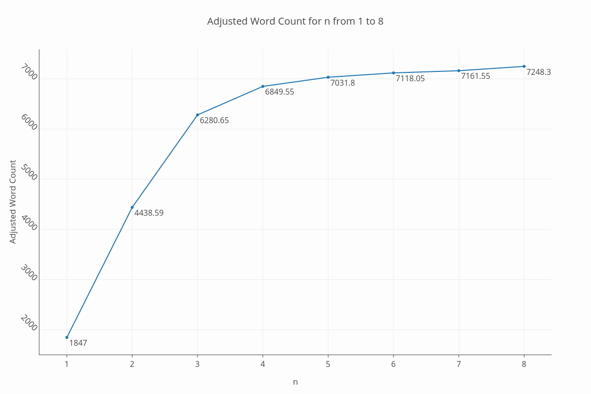
I did experiment with varying n, and the only significant effect besides changing the necessity of the graph filter was in the adjusted word counts. For example, at n = 8, the total adjusted word count jumps from about 7,000 to 7,200. This makes sense: if shared phrases are required to be longer, less of them will be identified and so the measurement of unique words will increase. Overall, there is no point in attributing more than one or two significant figures to that measurement because it depends so highly on your choice of n, but it does appear to converge between 7,000 and 7,500:

Conclusion

My two main goals for this project were to calculate an adjusted word count that accounts for essay reuse and to programmatically identify prompts that I was able to answer with the same essay. My total adjusted word count is equal to approximately 7,000 words, and two main groups of prompts were identified: “describe an extracurricular” and “explain your academic experience and goals as a student” (QED). These groups are extremely specific to me as a student, but I hope the results could help give insight into the process of applying to college, especially with respect to what colleges are actually asking for from their students.

If you are interested in hearing more about my experience addressing these prompts, check out Part 2, where I’ll talk about my approach to writing these essays and give tips based on this information. It will be much less technical and geared towards students preparing their own applications. I wish you all good luck!

Lastly, as I write this, almost all my applications are still in circulation, so as I wish you all luck I hope you can all reciprocate. I am nervous and excited about hearing the results.

Thanks for reading!