I love them, and I want you to love them too

There are a lot of machine learning techniques that have become fundamental tools for building more complex applications. Even though they’re individually complicated, most of them can be considered in terms of their ability to handle specific kinds of data, lending nicely to very simple and digestible abstractions. My goal for this post is to give an intuitive explanation of “word vectors,” and to break down the specific mechanics behind their creation.

In a nutshell, word vectors are important because they seem to represent the meaning of words in a numerical format that computers can analyze. Most students are introduced to vectors through school, and we all know the mantra: vectors have magnitude and direction. We usually see them visualized in relationship to an origin point, like a center:

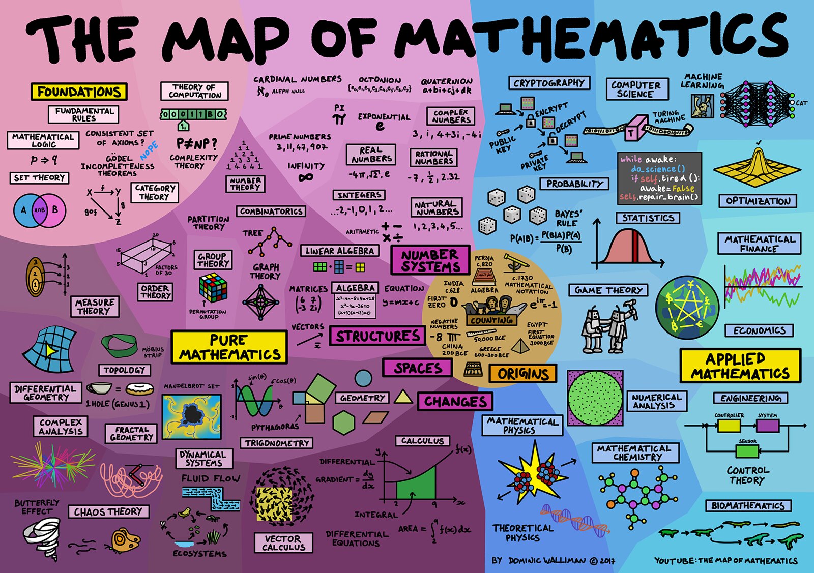
These vectors are all hanging out somewhere in the entire plane of space available to them. Using vectors to encode information means grouping them in that space so that the locations themselves are associated with some meaning. My favorite example of assigning meaning to different regions of space is the great Map of Mathematics, by Dominic Walliman – which I present with a wink to the top right corner. The great big idea around word vectors is that the algorithm finds a vector for each word so that similar words end up in similar places. This way, different regions of the space correspond to “similar meanings.”

Before explaining the process, I want to make one more point. Vectors don’t necessarily need to be in two dimensions. In fact, vectors can have an arbitrary number of dimensions, even though it becomes impossible to visually examine their magnitude and direction beyond three. Some vector operations, like the cross product, are only defined for a specific number of dimensions, but most vector operations are defined for arbitrary dimensions too. The dot product is a good example of an operation that extends well into multiple dimensions, and it’s important to this post. First off, the result of a dot product is a scalar, in contrast to the cross product which gives another vector. It is defined to be the magnitude of one input vector scaled by the length of another vector in the same direction. Like usual, this makes much more sense visually:

What’s important about the dot product is how many different ways you can compute one. The image above looks a bit like a triangle where one vector is the hypotenuse, demonstrating how the dot product can be defined in terms of the angle between the two vectors: $\vec{u} \cdot \vec{v} = \|\vec{u}\| \cos \theta$. If we define the two vectors in terms of their components, we can also just do the scaling by adding the products of each dimensions:

$\vec{u} = \begin{pmatrix} 80 \\ 60 \end{pmatrix}, \ \vec{v} = \begin{pmatrix} 150 \\ 0 \end{pmatrix} \\ \vec{u} \cdot \vec{v} = (80)(150) + (60)(0)$

Even I think it’s tedious to examine different ways to define the dot product, but there’s something important here. We’ve just established a relationship between the angle between two vectors, a visual indicator of their difference, and the process of summing the products of their components, which works in any number of dimensions. Most of the interesting aspects of word vectors are analyzed through vector similarity measurements, like “cosine similarity.” The cosine similarity is really just a measurement between 1 and -1 that expresses the cosine of the angle between them. Because of our component definition of the dot product, this distance measurement extends to higher dimensional vectors, even when angular distance might not make sense.

Why are they important?

Well, according to Google:

A non-obvious degree of language understanding can be obtained by using basic mathematical operations on the word vector representations.

Like a lot of those machine learning tools, word vectors are an idea that have been around for a while but recently became much more relevant when someone figured out a way to scale up the generation process. This time it was Google, in the link above. Specifically, Google researchers introduced the Word2Vec suite of algorithms that make it much faster to process larger sets of text. They also observed some interesting relationships between their vectors:

• Words that are contextually similar have similar vectors
• The distance between the vectors for analagous words is the same. For example, the paper lists the distance between “Montreal” and “Montreal Canadiens” as similar to the distance between “Toronto” and “Toronto Maple Leafs.”
• Finally, according to the paper the word vector sums can be useful as well. They use the example of the sum of “Russia” and “River,” which is close to “Volga River.”

These results have potential, to say the least. These examples alone indicate a level of semantic representation that has always seemed like the thing computers can’t do.

How are they generated?

There’s a simple fact about Word2Vec that I didn’t realize for weeks after I first understood the method. It’s very similar to an autoencoder! I’m going to introduce neural networks with an explanation of the autoencoder, and then step up to word vectors from there.

Crash Course on Neural Nets

Autoencoders are a specific type of “neural network.” Neural networks are mathematical models for biological neurons, which activate (put out an electrical impulse) when their inputs (other electrical impulses) are greater than the activation threshold. Mathematically, artificial neurons have numeric inputs and outputs, and the activation function can be a bit more complicated than a threshold. Like biological neurons, some input channels are more “important” than others, such that impulses of the same magnitude down different channels have different impacts on the activation threshold. There is also a “bias,” which is just an input that is constant and always active, allowing the activation function to be shifted left or right.

The neuron in the image above would use the following model: $i = x_1 w_1 + x_2 w_2 + b \\ o = f(i)$

What makes these neurons powerful is the ability to find optimal weights to get specific outputs from specific inputs. We do this by defining an error function in terms of the network’s output $o$ and the actual (or ideal) output $a$. For example, $E(o, a) = \|o - a\|$. Since we have already defined $o$ in terms of our weights, we can rewrite the error function as follows:

$E(x_1, x_2, a) = \| f(x_1 w_1 + x_2 w_2 + b) - a \|$

It is important to note that even though this is a function in terms of the inputs and outputs, we still have unknown variables: the parameters. Our goal is to find the parameters that minimize error given a specific set of inputs, so we can just substitute a set of inputs into the network and use calculus to do the minimization. This will involve taking partial derivatives of a multivariable function, which is actually really easy: all of the other variables are just considered to be constant. I’ll walk through the minimization process step by step, replacing constant terms with $c$.

• Collect all the inputs into a vector: $\vec{x} = \begin{pmatrix} x_1, & x_2, & ... & x_n, 1 \end{pmatrix}$
  The last component allows one of our weights to serve as our bias so that we don’t have to consider it separately.
• Collect all parameters into a vector: $\vec{w} = \begin{pmatrix} w_1, & w_2, & ... & w_n \end{pmatrix}$
• Redefine the network in terms of our new vectors: $o = f(\vec{x} \cdot \vec{w})$
  
• Now, for each of the weights, we want the rate of change of the error function with respect to that weight: $E(\vec{w}) = \| c - f(\vec{c} \cdot \vec{w}) \| \\ \frac{\delta E}{\delta w_i} = c f ' (cw_i + c)$
  Note that this requires the activation function to be differentiable, and ideally the derivative is efficient to calculate.
• In vector form, using the gradient: $\nabla E = \begin{pmatrix} \frac{\delta E}{\delta w_1}, & \frac{\delta E}{\delta w_2}, & ... & \frac{\delta E}{\delta w_n} \end{pmatrix}$
• Now, here’s the kicker. We’re going to scale the gradient down with a small positive constant $\eta$, which is chosen arbitrarily. Then, we subtract the scaled error gradient from the weights. Each weight is shifted in the opposite direction of the rate of change of error for that weight. $\vec{w_{n}} = \vec{w_{o}} - \eta \nabla E$

The subscripts in the last step indicate new and old weights, or those that come before and after the shift. During the shift, if error increases when the weight increases, the rate of change is positive and so that weight is decreased, and vice versa when error decreases. If we repeat this process for tons of examples, we “learn” weights that approximate the ideal outputs for tons of different inputs.

In practice, there are a few important architecture decisions to make that I want to mention for completeness’s sake. Like the brain, we can introduce extra neurons, that each receive the same input $\vec{x}$ but that have different weights. A group of neurons that all receive the same inputs is called a “layer.” We can also introduce extra layers, where the “first” layer has input $\vec{x}$ and output $\vec{o_1}$, the “second” layer has input $\vec{o_1}$ and output $\vec{o_2}$, and so on. Finally, activation and error functions are almost never as simple as the ones I used here. These are generally chosen to fit the data itself, with consideration also put towards the efficiency of calculating that function.

This process is definitely complicated, but the key takeaway is that we can use lots of input output examples to find weights for a neural model to approximate that data.

The Autoencoder

Up to this point, we’ve considered neural networks in terms strictly numeric inputs, but it’s important to understand that these aren’t just arbitrary numbers – they generally represent an actual entity. For example, a network might take inputs like the size of a house, the number of bathrooms, or the number of rooms to predict the house’s price. Because each of these aspects of the house serve as inputs to the network, we can shift our focus to $\vec{x}$, which serves as a “computer readable” proxy for the real-world, semantic idea of the house itself. It is the amalgamation of our objective evidence about the house, and our goal is to learn the complex relationship between that evidence and our ideal output. This is another important idea: we can use vectors to represent the “important” characteristics of real-world entities. The goal of the autoencoder is to find a compressed representation (ie. one with fewer dimensions) to best capture the input.

An standard autoencoder has two “layers.” The input has $d_i$ components (the “input dimensionality”) such that $\vec{x} \in \mathbb{R}^{d_i}$ (the input exists in the $d_i$ dimensional set of real numbers). The first layer has fewer neurons than inputs and the last layer has $d_i$ output nodes. Then, the error function is just the difference between the output and the input. So, the network has to learn the “most important information” to compress into the small layer’s output so that it can reconstruct the original input from that information. Here is an example:

An autoencoder’s accuracy depends highly on the size of the input vector and the number of neurons in the first layer, but it also depends highly on the redundancy of the data itself. Imagine a set of 4-dimensional input data examples where there is a very high change that the first three values are the same for any input case. Since those three are generally redundant, the input data could be collapsed from four to two dimensions without losing much accuracy. THe autoencoder encoder allows you to compress (or “encode”) data into fewer dimensions by eliminating redundancy.

Autoencoding Words

As with the house example, we need to come up with representative vectors for words before we can use them in a neural network. We do this by establishing $V$, the size of our vocabulary, and then assigning the $n$th word a $V$ dimensional vector in which the $n$th component is $1$ and the rest are $0$. Basically, each word gets a specific dimension indicated by the $1$ component. These are called “one-hot” vectors, and the reason for this encoding scheme will become clear later.

Our data source is just a ton of text – the more the better. Instead of using one of these words as inputs and trying to get it back as output, we’re going to try to use the word’s context. At this point, Google provides two similar approaches to accomplishing this goal. For simplicity, I’ll focus on one before the other: the “skip-gram” model. If you’ve read this previous post you’ve already heard of the n-gram: an ordered collection of $n$ words. A skip-gram is like an n-gram, but one word is skipped. A example skip gram from the first five words of this sentence is (an, example, _, gram, from). In the skip gram model, the user sets the target dimensionality $d_t$ and the goal is to reconstruct the skip gram given the missing word. With the example above, the word “skip” would be converted to its representative vector and given as input to $d_t$ neurons. Then, an output layer of $V$ neurons should reconstruct a vector in which ideally every component is $0$ except for the components corresponding to “an,” “example,” “gram,” and “from.”

Where an autoencoder was simply learning to create a compressed encoding for the data, this network is taking every word’s context and compressing that. Because we originally used one-hot vectors, only the weights corresponding to the $n$th input (the only $1$ in our input vector) matter, because the other weights are multiplied by zero. So, we have $d_t$ non-trivial weights, and we’re looking for a representative vector with $d_t$ components… We’ll just group them into a vector – and that’s the word vector.

Even in their paper, the authors express some surprise that the method works. The input values to a network trained to reconstruct context serve as a representation of that word’s context. This is how the word vectors are generated – QED. In the other model for training word vectors, the input is the sum of all of the one-hot vectors for the context words, and the network is trained to output whatever word is missing. This is called the “Conditional Bag of Words” model (CBOW), because the goal is to estimate the conditional probability of a single word given the unordered collection of context words, as if your network is an actual bag of jumbled context words. This is actually just the architectural opposite of the skip-gram model, and both relate one word to those which are likely to appear near it. In both cases, the same goal is accomplished: the weights to the first layer serve as vector representations of the vocabulary words.

Conclusion

In summary, the Word2Vec generation process can be summarized in a few steps: given a large data set of words, try to learn vector representations for each word such that the context can be reconstruct with the most accuracy using just that vector representation. It is interesting to note that all of that contextual information is extracted from patterns of word occurences, and nothing else. These representations have been widely used as more informative surrogates for words in a dataset, and they frequently take the place on one-hot word inputs in “downstream” applications (those which happen after the word vectors are generated for the corpus). Because this technique is so versatile, it is an important and fundamental tool in machine learning that allows computers to operate on the contextual relationships between words in a dataset.