This post is short because I’ve been distracted by final exams, which are all in May. There probably won’t be a post in May for the same reason.

Image convolutions are a foundational tool in many machine learning based computer vision tools today. They were introduced as a general purpose image processing technique, and along with pooling layers they provide a natural way for neural networks to simplify image input and avoid learning weights for every single pixel. If you’re not familiar with them already, I recommend this page for an introduction.

The basic benefit of image convolutions is that they provide a numeric structure that can isolate features of an image. Convolutions can, for example, isolate edges, patterns of color, or sharpen parts of an image – this is why they see use in image processing. In machine learnine, this information is extremely useful for understanding which parts of an image are important and which aren’t. Convolutions also reduce the number of parameters, which can help avoid overfitting and reduce training times. Because of their benefits the technique has become a foundational technique in computer vision and machine learning.

As in the tutorial above, many explanations of convolutions simple demonstrate how they get applied to a grey scale image. The process is fairly intuitive, especially when animated, and so it’s easy to understand how convolutions are applied. Many tutorials unfortunately don’t cover how convolutions are applied to feature maps with multiple channels. For example, knowing how I can apply a convolution to a single greyscale image is helpful, but how do I apply that knowledge to an image with red, green, and blue channels?

Many sources will demonstrate their architectures using a diagram like this, from the DCGAN paper.

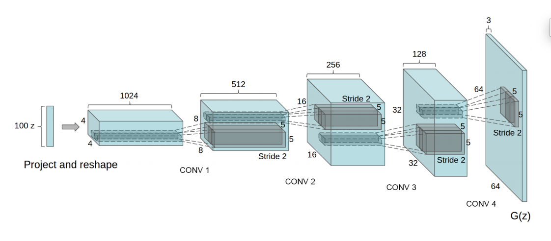
This is a helpful image if you already understand how convolutions operate on multi-channel feature maps, but one of my biggest difficulties in understanding papers like the one above was finding a good explanation for that operation. Most tutorials either assume it follows naturally from a single channel or provide a dense and non-visual definition for the general convolution operator.

The most authoritative source I know on machine learning implementations is the Tensorflow Documentation, which says this:

output[b, i, j, k] = sum_{di, dj, q} input[b, strides[1] * i + di, strides[2] * j + dj, q] * filter[di, dj, q, k]

This falls into the category of dense explanation, but if we pick it apart it’s not so complicated. First off, we can ignore $b$ because it gives the index of an image in a minibatch. A pixel in a multichannel feature map has three coordinates, $i$, $j$, and $k$. $k$ corresponds to a specific output channel, and $i$ and $j$ correspond to a pixel in that chanel. $q$ corresponds to a specific input channel. $di$ and $dj$ correspond to the indexes surrounding the pixel $(i, j)$ which are relevant to the convolution. $\sum_{di,dj,q}$ means “for every pixel in the vicinity of $(i, j)$ in any of the input feature maps,” and the body of that summation multiplies each specific pixel in each feature map by filter[di, dj, q, k]. This is the specific convolution weight corresponding to a vicinity pixel for a specific input $q$ and output $k$. So, for every output channel $k$, there is one convolution for ever input channel $q$. The results of all the convolutions across all the feature maps get summed into a single value that makes up a pixel in the output. This is how convolutions apply to feature maps with multiple channels.

Unfortunately, even my attempt at a clearer definition is still dense. See this diagram for a visual explanation of the process:

Convolutions applied to each input channel make up the pixels of a single output channel. That’s the key takeaway for this post.